Graphical User Interface
The Waveform Editor provides a Graphical User Interface (GUI), with which you can:
Create, load, edit, and save waveform configurations from YAML files.
View plots of one or multiple waveforms simultaneously for comparison.
Edit waveforms through a text editor with live plot updates and error highlighting.
Export waveform data to various formats, including IDS, CSV, PNG, and PCSSP XML.
Graphically edit and design the desired plasma shape using NICE.
Launching the GUI
The GUI can be launched using the following command in your terminal:
waveform-editor gui
You can also optionally specify a YAML file to load on startup:
waveform-editor gui /path/to/your/waveforms.yaml
Note
This normally opens automatically in your default web browser. If it does not,
you can manually open the app in a web browser by going to the address printed in the terminal.
For example, when the waveform-editor gui command has the following output, the app is running
on the web address http://localhost:38895.
$ waveform-editor gui
[...]
Launching server at http://localhost:38895
File Handling
All file operations are managed through the File menu located at the top of the
sidebar. This menu allows you to create, open, save, and export waveform
configurations. The name of the currently open file is displayed next to the menu.
An asterisk (*) next to the filename indicates that there are unsaved changes.
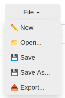
File Menu Interface
Opening a Configuration file
You can start a new configuration or open an existing one from the sidebar's File menu.
To start a new, empty waveform configuration, click File > ✏️ New.
To load an existing waveform configuration from a YAML file, click File > 📁 Open.... This will open a file dialog where you can navigate to and select your
.yamlfile.
Saving a Configuration
You can save your work in two ways:
File > 💾 Save: This option saves the current configuration to the currently open file. If you are working on a new, untitled configuration, it will trigger the "Save As" dialog instead.
File > 💾 Save As...: This opens a file dialog, allowing you to save the current configuration to a new file or overwrite an existing one.
Exporting a Configuration
To export the waveform data, click File > 📤 Export.... This opens the export dialog, which provides several options:
Output type: Choose the desired format for the export.
IDS: Exports the data to an IMAS database entry. You must provide a valid IMAS URI.
CSV: Exports all waveforms into a single CSV file, with a time column and a column for each waveform. You must provide a valid output file path.
PNG: Exports a plot of each waveform as a separate PNG image file. You must provide a path to an output directory.
PCSSP XML: Exports the data into the PCSSP XML format.
Time Options: Define the time points at which the waveforms will be evaluated. This is required for all export types except PNG with the "Default" option.
Default (only when exporting to PNG): Each waveform is plotted using its own automatically determined time array.
Linspace: Creates a linearly spaced time array from a Start time, Stop time, and the Number of points.
CSV File: Upload a CSV file containing a single row of comma-separated time values.
Manual: Manually enter a comma-separated list of time values (e.g.
0, 0.5, 1.0).
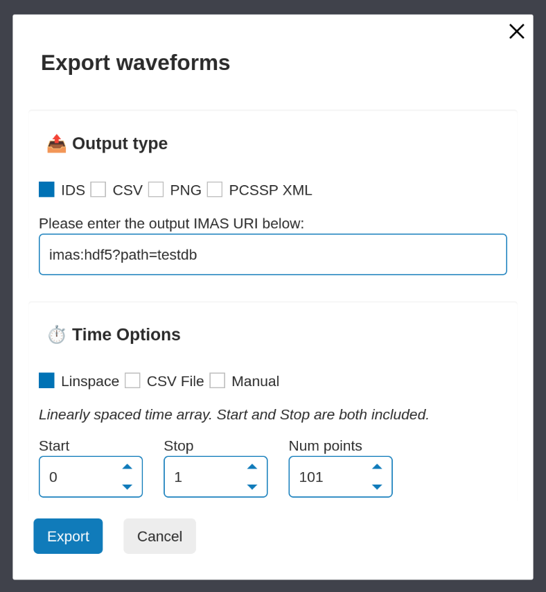
The export dialog
Editing Configuration
The main interface is divided into a sidebar for selection and a tabbed area for viewing and editing. The workflow involves selecting waveforms in the sidebar and then using the tabs to view or modify them.
Waveform Selection Options
The waveforms in the configuration are organized into hierarchical structure of groups, For more details on the file format, see the YAML File Format section. This structure is visualized in the sidebar of the GUI.
For each group, a row of buttons provides several actions:
 (Add new waveform): Creates a new, empty waveform within that group.
 (Remove selected waveforms): Deletes all selected waveforms within that
group.
(Remove selected waveforms): Deletes all selected waveforms within that
group. (Add new group): Creates a new subgroup.
 (Select all): Selects all waveforms in the group (only available in the
"View Waveforms" tab).
(Select all): Selects all waveforms in the group (only available in the
"View Waveforms" tab). (Deselect all): Deselects all waveforms in the group.
 (Remove this group): Deletes the group and all its contents (waveforms and
subgroups).
(Remove this group): Deletes the group and all its contents (waveforms and
subgroups). (Rename waveform): Renames the single selected waveform in that group.
Filtering Waveforms
To quickly find specific waveforms in large configurations, a filter bar is available at the top of the waveform selector sidebar.
As you type into the "Filter waveforms..." box, the waveforms will be filtered based on whether the names contain the typed text. The search is case-insensitive.
To return to the tree view, you can either clear the text from the filter bar
manually or click the Clear filter (![]() ) icon that appears next to it.
) icon that appears next to it.
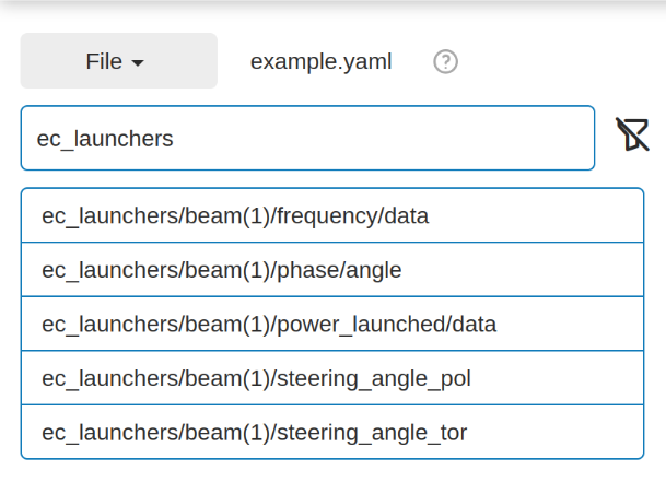
Filtering waveforms containing ec_launchers
for this example configuration
Viewing and Editing Waveforms
The GUI provides two main tabs for working with waveforms: View Waveforms, and Edit Waveforms.
The View Waveforms tab allows you to plot multiple waveforms on the same axes for comparison. In this mode, you can select multiple waveforms from the sidebar, and they will be displayed in the plot on the right.
The Edit Waveforms tab is designed for modifying a single, selected waveform. This view is split into two sections:
Code Editor: The YAML definition for the selected waveform is displayed here. You can directly edit the text, and the plot will update automatically. If there are syntax errors or inconsistencies in the waveform logic, an error or warning message will appear below the editor, and annotations will highlight the problematic lines.
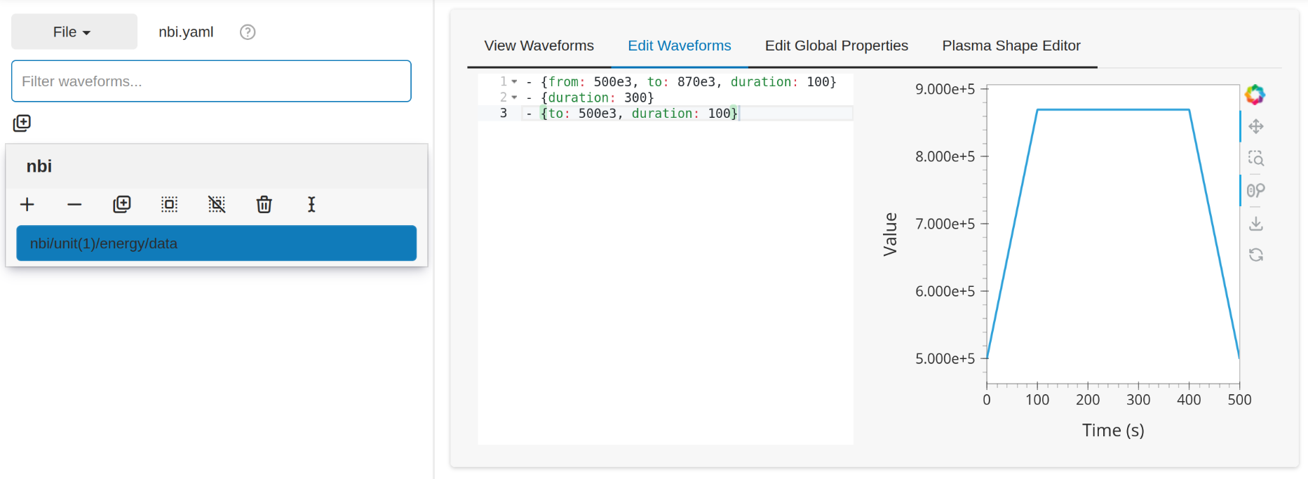
Example of an nbi waveform, showing the code editor containing the waveform YAML defition, and the plot showing the waveform currently being editted.
Interactive Plot: For waveforms with
piecewisetendencies, the waveform can be updated by interacting with the plot. All changes are instantly reflected in the YAML code. To interact with the plot, ensure you enable the Point Draw Tool ( ).
You can:
).
You can:Add Points: Click anywhere on the plot to add a new point. Note: it is not possible to interactively add points before a piecewise tendency, or between two different piecewise tendencies.
Move Points: Select one or more point and drag to change their time and value.
Remove Points: Select one or more points and press Backspace.
Editing Global Properties
The Edit Global Properties tab allows you to configure settings that apply to the entire configuration. Changing these updates the global properties of the configuration. Information about the avilable properties can be found in the Global properties section.
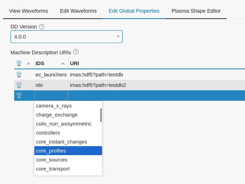
Example showing how to set the global properties
Plasma Shape Editor
The Plasma Shape Editor provides an interactive interface for running the NICE (Newton direct and Inverse Computation for Equilibrium) solver. This allows you to design and analyze plasma equilibria by either specifying a desired shape and finding the necessary coil currents (Inverse Mode) or by providing coil currents and calculating the resulting plasma shape (Direct Mode).
The interface is primarily divided into two sections: a large plotting area on the left that displays the machine geometry and equilibrium results, and a control panel on the right with various configuration options.
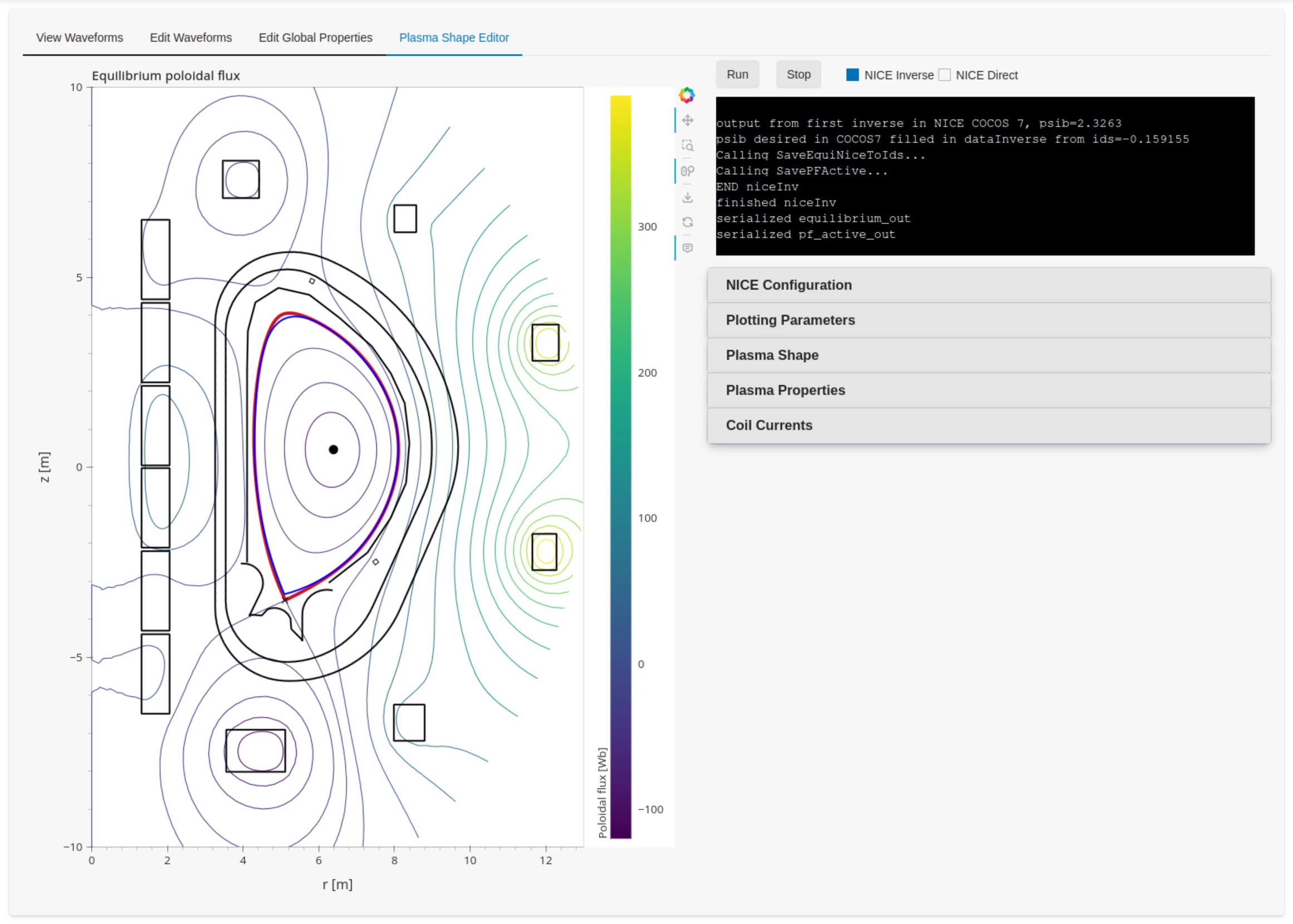
Overview of the Plasma Shape Editor
Operating Modes
NICE can be run in two modes, which can be selected using the radio buttons at the top of the control panel:
Inverse Mode: You define a target plasma shape and properties, and NICE calculates the required coil currents to achieve this equilibrium. You can also choose to fix the current in a subset of coils.
Direct Mode: You specify the currents for all coils, and NICE calculates the resulting plasma equilibrium.
At the top of the control panel, you'll find Run and Stop buttons to start and terminate the NICE simulation. A terminal window below these buttons displays live output from NICE.
Configuration Options
The control panel on the right contains several collapsible option menus, each dedicated to a specific part of the configuration. A warning icon (⚠️) next to a option title indicates that required information for this section is missing, and needs to be updated for NICE to run.
The following option menus are available, these will be explained in detail in the sections below:
NICE Configuration: Required NICE configuration parameters.
Plotting Parameters: Configuration for the plot.
Plasma Shape: Target plasma shape when running NICE in Inverse Mode.
Plasma Properties: Plasma characteristics, such as plasma current and p' / ff' profiles.
Coil Currents: The currents through the active field coils.
NICE Configuration
This is where you set up the core parameters for NICE and provide the necessary machine description files.
This section includes settings for:
The file paths to the NICE executables for both inverse and direct modes. If you are using the NICE module, you can leave these at their default values:
nice_imas_inv_muscle3andnice_imas_dir_muscle3. If you manually built NICE, these should point to the executables that were built in this section. For example:path/to/nice/run/nice_imas_inv_muscle3andpath/to/nice/run/nice_imas_dir_muscle3for the inverse mode and direct mode executable paths respectively.Any environment variables that NICE requires. These are stored as a dictionary of strings. For example:
{'LD_LIBRARY_PATH': '/home/user/.local/lib'}The IMAS URIs for the machine descriptions.
The level of detail in the output logs generated by the solver.
Note
The settings in the NICE Configuration section are persistent. They are
automatically saved to a configuration file (by default located in $HOME/.config/waveform_editor.yaml)
and will be reloaded each time you start the application.
Plotting Parameters
This contains options to change the visualization in the plotting area. You can show/hide all the different plotting elements, and choose how many contour levels to use for plotting the poloidal flux.
Plasma Shape
This option is only available in Inverse Mode and is used to define the target plasma boundary. There are three methods for specifying the shape:
Equilibrium IDS outline: Loads the plasma boundary outline directly from a specified time slice of an existing equilibrium IDS.
Parameterized: Generates a parameterization of the shape based on a set of geometric parameters.
Equilibrium IDS Gaps: Loads gaps from an equilibrium IDS. The distance value from the reference point can be changed from the UI.
Plasma Properties
This contains settings for configurating the plasma's physical properties. You can either load them from an existing equilibrium or define them manually.
Equilibrium IDS: Loads the plasma current (Ip), reference major radius (R0), toroidal field (B0), and the p' and ff' profiles from a specified time slice of an equilibrium IDS.
Manual: Allows you to set Ip, R0, and B0 manually. The p' and ff' profiles are configured using the alpha, beta, and gamma parameters as described below.
Here, \(\psi_N\) is the normalized poloidal magnetic flux, \(r_0\) is the major radius of the vacuum chamber, and \(\mu_0\) is constant magnetic permeability of vacuum. Note, the actual p' and ff' will be scaled by NICE to satisfy the required total plasma current Ip.
The parameter beta is related to the poloidal beta, whereas alpha and gamma describe the peakage of the current profile. See equation 2.11 in B. Cédric, et al. "CÉDRÈS: a free-boundary solver for the Grad–Shafranov equation." (2014)
Coil Currents
This allows you to view and control the currents in the coils defined in the pf_active IDS. Its behavior changes depending on the operating mode:
In Inverse Mode, each coil has a checkbox and a slider. If you check the box next to a coil, its current is fixed to the value set by the slider. Unchecked coils are free to change and their currents will be calculated by NICE. After a successful run in Inverse Mode, the sliders will be updated to show the calculated currents.
In Direct Mode, the sliders for all coils are enabled. You must use these sliders to provide the input current for every coil.
You can save the coil currents to waveforms at a chosen export time. The coil current
values will be stored in a Piecewise Linear Tendency at the end of the
corresponding waveforms (for example: pf_active/coil(1)/current/data). This allows for a
convenient construction of a waveform by iteratively executing the following:
Configure the plasma parameters and shape.
Execute NICE to calculate the set of coil currents.
Set an export time value, and append the calculated values to their respective waveforms.