Training¶

In order to start editing waveforms, you must first learn how to navigate your way around the GUI. Launch the Waveform Editor GUI using the following command, which opens the Waveform Editor in your default browser.

waveform-editor gui

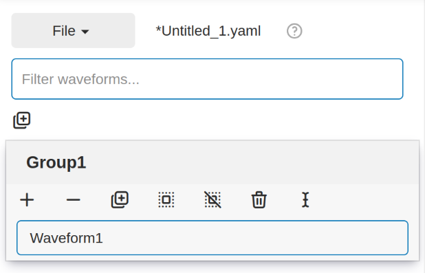
1. A waveform must always belong to a group, so first use this button in the sidebar to create a group in which to store the new waveform, and provide a name for the group, e.g. Group1.

2. Use this button to create a new waveform in the previously created group, and provide a name for this waveform, e.g. Waveform1.

What do you see in the sidebar on the left?

You have now created a new waveform, which is shown in the sidebar:

Now you will edit the empty waveform you created in the previous exercise. Select the waveform in the sidebar and open the Edit Waveforms tab. You will see an editor window as well as a live view the waveform currently being edited.

The editor currently shows - {}, indicating an empty tendency. A tendency can be specified by providing a tendency type and by setting parameters defining the shape of this tendency. For example:

- {type: <waveform type>, <param 1>: <value 1>, <param 2>: <value 2>, ...}

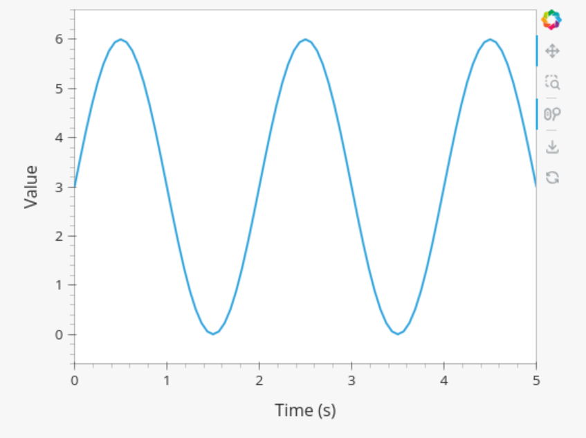
Edit the waveform you created in the previous exercise such that it contains a single sine-wave tendency, with the following parameters:

• Type: sine

• Duration: 5 seconds

• Frequency: 0.5 Hz

• Amplitude: 3

• A base offset of 3

Use the following tendency parameters: type, duration, frequency, amplitude, and base.

1. Switch to the editor tab and edit the waveform. Enter the following into the editor:

- {type: sine, duration: 5, frequency: 0.5, amplitude: 3, base: 3}

You should see the following waveform:

In the previous execise, you might have noticed that there a multiple ways in which you can define the same waveform. Recreate the waveform of previous exercise using only the following tendency parameters: type, duration, period, min, and max.

The resulting waveform should be:

- {type: sine, duration: 5, period: 2, min: 0, max: 6}

What happens if you overdetermine your waveform? For example, set both the frequency, as well as the period of the sine wave: frequency: 0.5 and period: 2

And what happens if frequency and period would result in a different sine wave? For example, set frequency: 2 and period: 2?

If you set the frequency: 0.5 and period: 2, since these do not conflict, this waveform is allowed.

- {type: sine, start: 10, duration: 5, frequency: 0.5, period: 2, min: 0, max: 6}

If you set the the frequency: 2 and period: 2, for example:

- {type: sine, start: 10, duration: 5, frequency: 2, period: 2, min: 0, max: 6}

you will see an error pop up in the editor, notifying you that the period and frequency do not match.

In the previous exercises, you created a waveform that contained only a single tendency. However, waveforms can contain any number of tendencies, by adding additional lines in the editor.

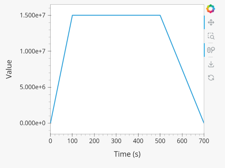
We will now design a simple waveform representing the plasma current during a single pulse. Create a waveform called equilibrium/time_slice/global_quantities/ip, which has the following shape:

1. A linear ramp up from 0 to 15e6 A, in a duration of 100 seconds (use tendency type: linear).

2. A flat-top at 15e6 A, held for 400 seconds (use tendency type: constant).

3. A ramp down back to 0 A, in a duration of 200 seconds (use tendency type: linear).

A possible list of tendencies for this waveform can be:

- {type: linear, from: 0, to: 15e6, start: 0, duration: 100}
- {type: constant, value: 15e6, start: 100, duration: 400}
- {type: linear, from: 15e6, to: 0, start: 500, duration: 200}

You should see the following waveform:

In the previous exercise, the solution proposed was very quite lengthy. The Waveform Editor can sometimes deduce some information about the tendencies if information is missing.

Some examples:

1. If no start parameter is provided, the end of the previously tendency will be used as a start value, or 0 if it is the first tendency.

2. If no tendency type is provided, it will be considered a linear tendency by default.

3. If no start value e.g. from is provided, it will try to match end of previous tendency.

Replicate the waveform in the previous exercise using this shortform notation.

In the shortform notation:

1. The first tendency - No start or from is needed because it begins at 0 by default.

2. The second tendency - No type is provided, so it is a linear tendency by default. The start, from, and to parameters are by default set to the respective values at the end of the previous tendency.

3. The third tendency - Again, the start and from parameters are inferred from the previous tendency. In this case, we do need to specify the to parameter, otherwise we would get a straight line.

- {to: 15e6, duration: 100}
- {duration: 400}
- {to: 0, duration: 200}

Create a waveform that consists of the following two tendencies:

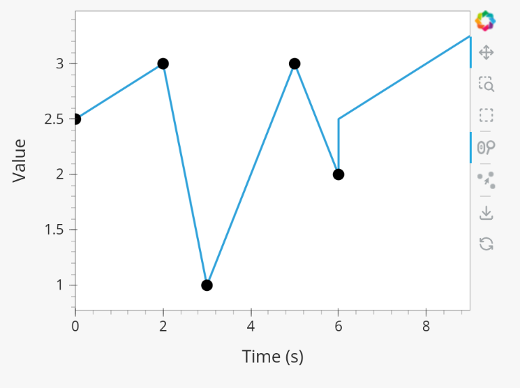
1. A piecewise linear tendency containing the following 5 pairs of points: (0,2.5), (2,3), (3,1), (5,3), (6,2)

2. A linear tendency starting from 2.5, with a rate of change of 0.25, lasting 3 seconds.

Your waveform can contain for example the following tendencies:

- {type: piecewise, time: [0, 2, 3, 5, 6], value: [2.5, 3, 1, 3, 2]}
- {type: linear, from: 2.5, rate: 0.25, duration: 3}

You should see the following waveform:

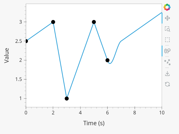
Continuing from the waveform in the previous exercise, modify it to include a smooth tendency with a duration of 1 between the two tendencies. What do you notice?

Your waveform can contain for example the following tendencies:

- {type: piecewise, time: [0, 2, 3, 5, 6], value: [2.5, 3, 1, 3, 2]}
- {type: smooth, duration: 1}
- {type: linear, from: 2.5, rate: 0.25, duration: 3}

You should see the following waveform. Notice how the smooth tendencies ensure continuous value and derivative across multiple tendencies.

You can create repeating patterns using the repeat tendency. This tendency allows you to specify the waveform parameter, here you can provide a list of tendencies that will be repeated for a length of time.

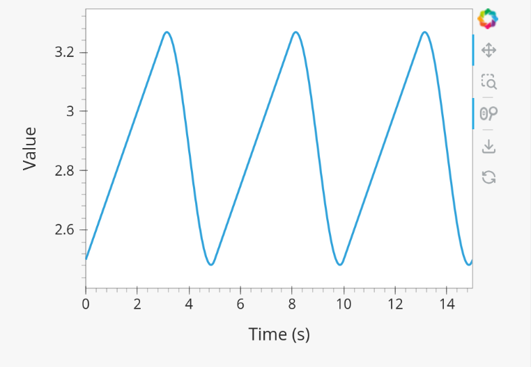
Copy the tendency list given below and use a repeat tendency to make it repeat three times.

- {type: linear, from: 2.5, rate: 0.25, duration: 3}
- {type: smooth, duration: 2}

The provided tendency list can be placed as is in the waveform parameter of the repeat tendency. Since the tendencies combine up to a total length of 5, the total duration of the repeat tendency is set to 15, to obtain three full cycles.

- type: repeat
  duration: 15
  waveform:
  - {type: linear, from: 2.5, rate: 0.25, duration: 3}
  - {type: smooth, duration: 2}

You should see the following waveform:

Waveforms can depend on other waveforms, and you can even perform calculations using other waveforms. In this exercise, you will define simple waveforms for the power of the electron cyclotron (EC) launchers.

The goal is to create:

1. A waveform total_power containing the total power of all EC launchers, this consists of a waveform that linearly ramps up from 0 to 5e5 W for 100 seconds, then flat-tops for 500 seconds, and finally linearly ramps down for 100 seconds.

2. We take 10 different beams, and define the derived beam power waveforms ec_launchers/beam(1:10)/power_launched/data that evenly divides the total power over each beam.

What happens to the derived waveform when you change the total power waveform?

Before starting with Exercise 4b, save the configuration containing the two created waveforms to disk. This will be used in a later exercise. To see how to save a configuration, have a look at the instructions.

Create a new waveform called total_power which contains:

- {type: linear, to: 5e5, duration: 100}
- {type: constant, duration: 500}
- {type: linear, to: 0, duration: 100}

Create a second waveform called ec_launchers/beam(1:10)/power_launched/data, this represents the power_launched for each of the ten beams, which contains:

"total_power" / 10

You should have the following two waveforms:

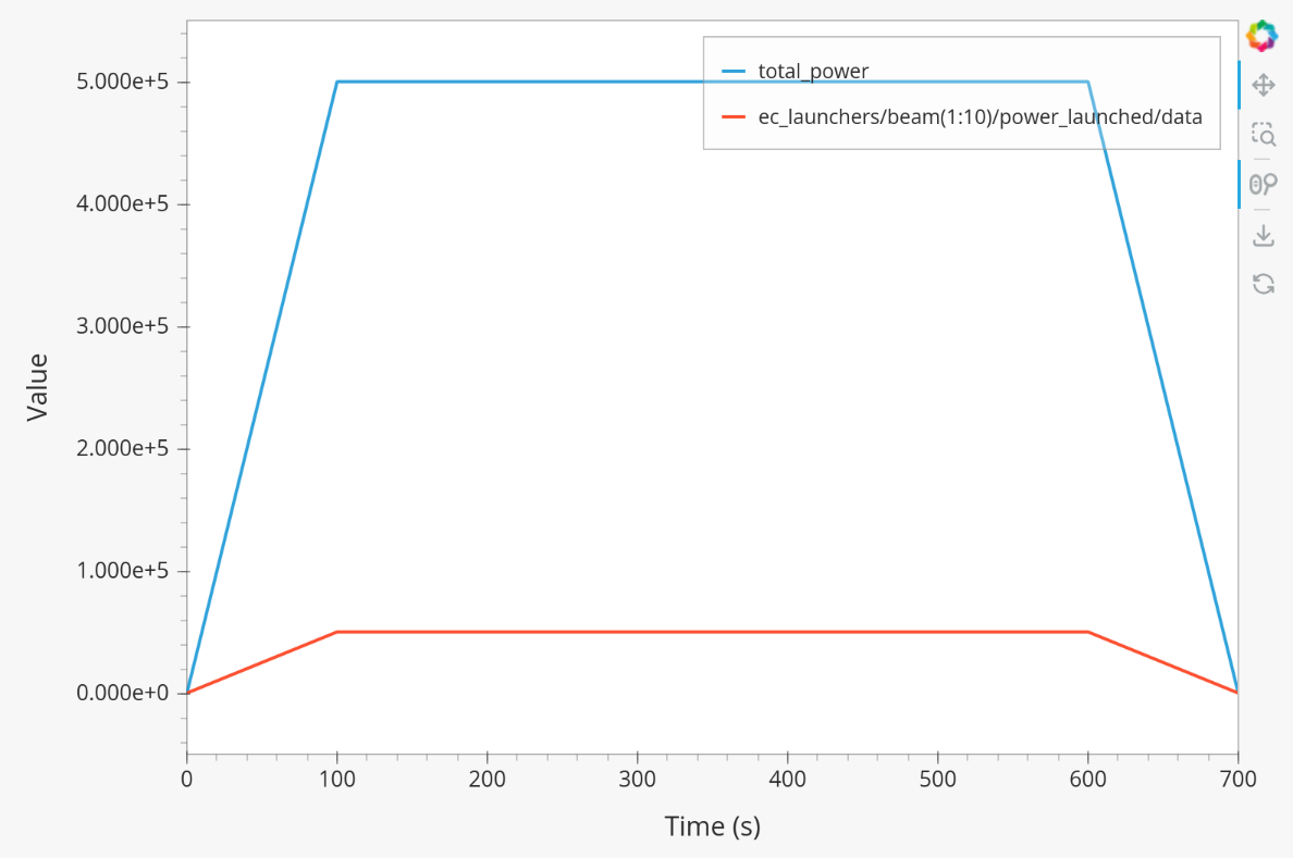
If you change the total_power waveform you should see that the derived waveforms changes as well.

In this exercise, you will define a derived waveform in which the Neutral Beam Injection (NBI) launch power depends on the beam energy through the following relation.

where:

• \(P_0\) = 16.5e6 W (nominal power per beam box)

• \(E_0\) = 870e3 eV (reference beam energy for hydrogen)

• \(E_\mathrm{beam}\) is the beam energy

Define the following waveforms:

1. nbi/unit(1)/energy/data - linear ramps up from 0 to 500e3, for 100 seconds, then flattops for 500 seconds, and then linearly ramps down for 100 seconds.

2. nbi/unit(1)/power_launched/data - derived from the energy using the above equation.

Create a new waveform called nbi/unit(1)/energy/data which contains:

- {type: linear, to: 500e3, duration: 100}
- {type: constant, duration: 500}
- {type: linear, to: 0, duration: 100}

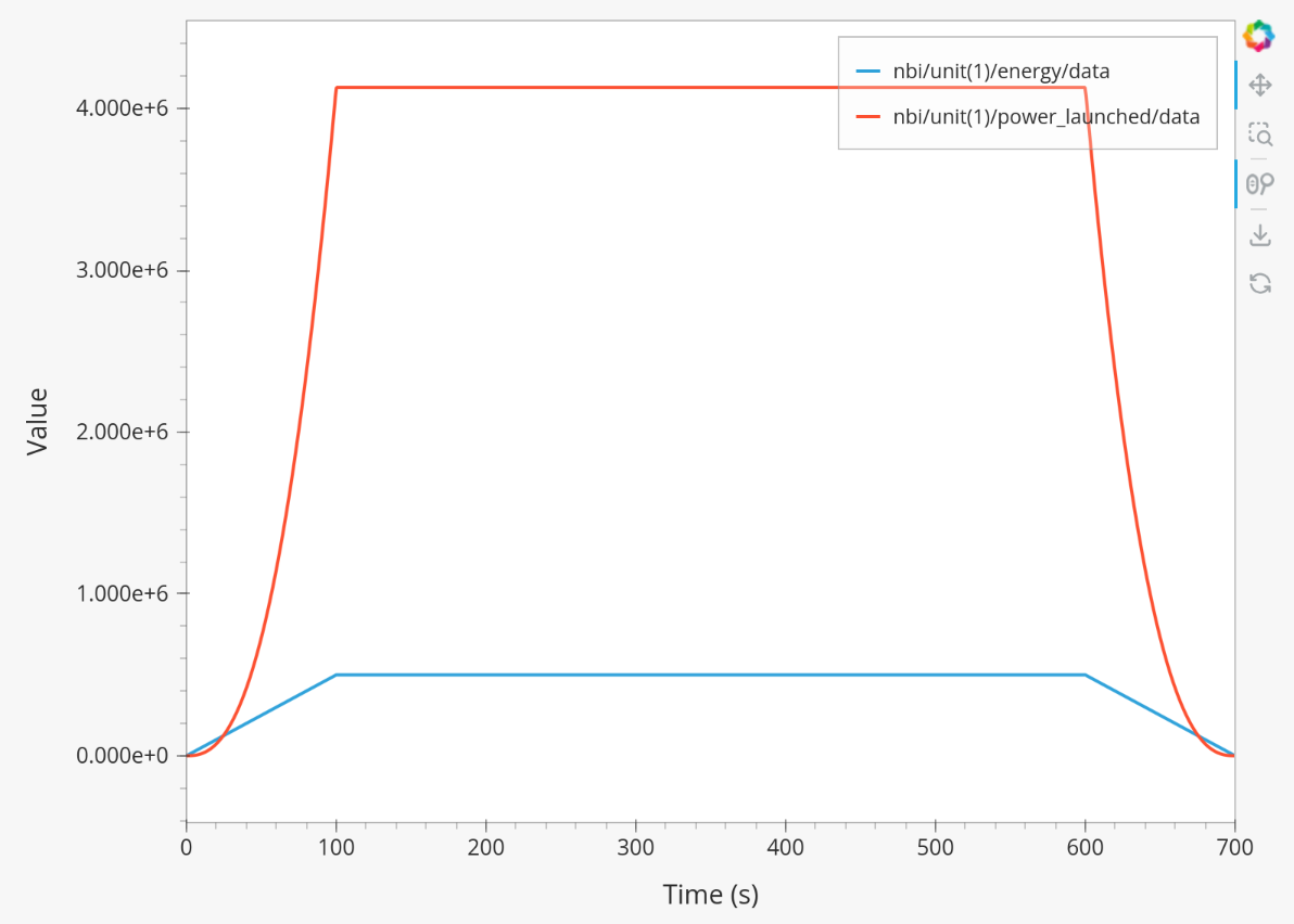
Create a second waveform called nbi/unit(1)/power_launched/data, which contains:

16.5e6 * ("nbi/unit(1)/energy/data" / 870e3) ** 2.5

You should have the following two waveforms:

In this exercise, we will continue with the configuration that you stored in exercise 4a. If you forgot to save it, the YAML is also shown under the tab Configuration. Load this configuration into the Waveform Editor, if you are unsure how to, have a look at the instructions here.

We will export our EC beam power values to an ec_launchers IDS, and store it using an IMAS NetCDF file. You can export to a NetCDF file by providing the URI in the following format: path/to/file.nc. Sample the time such that there are 20 points in the range from 0 to 800s.

Inspect the exported IDS using imas print <your URI> ec_launchers, which quantities are filled? Notice that the waveform in the configuration runs from 0 to 700s, while you export from 0 to 800s . What happens with the exported values outside of the waveform (time steps later than 700 s)?

If you forgot to save the configuration of exercise 4a, copy the following YAML file, and store it to disk and load it back into the waveform editor.

globals:
  dd_version: 4.0.0
  machine_description: {}
ec_launchers:
  total_power:
  - {type: linear, to: 5e5, duration: 100}
  - {type: constant, duration: 500}
  - {type: linear, to: 0, duration: 100}
  ec_launchers/beam(1:10)/power_launched/data: |
    "total_power" / 10

Printing the exported ec_launchers IDS shows the output below. Notice how the time array is filled with values from 0 to 800. The Waveform Editor will only export waveforms which name matches a path in the IDS. Therefore, the total_power waveform will not be exported to an IDS. Since we use a slicing notation for the power_launched waveform (beam(1:10)), the first 10 beams are filled with the same waveform.

Any values which are outside of the defined waveform range (e.g. values later than 700s) will be set to 0.

ec_launchers
├── ids_properties
│   ├── homogeneous_time: 1
│   └── ids_properties/version_put
│       ├── data_dictionary: '4.0.0'
│       ├── access_layer: '5.4.3'
│       └── access_layer_language: 'imas 2.0.1'
├── beam[0]
│   └── beam[0]/power_launched
│       └── data: array([    0.    , 21052.6316, 42105.2632, ...,     0.    ,     0.    ,     0.    ])
├── beam[1]
│   └── beam[1]/power_launched
│       └── data: array([    0.    , 21052.6316, 42105.2632, ...,     0.    ,     0.    ,     0.    ])
├── beam[2]
│   └── beam[2]/power_launched
│       └── data: array([    0.    , 21052.6316, 42105.2632, ...,     0.    ,     0.    ,     0.    ])
├── beam[3]
│   └── beam[3]/power_launched
│       └── data: array([    0.    , 21052.6316, 42105.2632, ...,     0.    ,     0.    ,     0.    ])
├── beam[4]
│   └── beam[4]/power_launched
│       └── data: array([    0.    , 21052.6316, 42105.2632, ...,     0.    ,     0.    ,     0.    ])
├── beam[5]
│   └── beam[5]/power_launched
│       └── data: array([    0.    , 21052.6316, 42105.2632, ...,     0.    ,     0.    ,     0.    ])
├── beam[6]
│   └── beam[6]/power_launched
│       └── data: array([    0.    , 21052.6316, 42105.2632, ...,     0.    ,     0.    ,     0.    ])
├── beam[7]
│   └── beam[7]/power_launched
│       └── data: array([    0.    , 21052.6316, 42105.2632, ...,     0.    ,     0.    ,     0.    ])
├── beam[8]
│   └── beam[8]/power_launched
│       └── data: array([    0.    , 21052.6316, 42105.2632, ...,     0.    ,     0.    ,     0.    ])
├── beam[9]
│   └── beam[9]/power_launched
│       └── data: array([    0.    , 21052.6316, 42105.2632, ...,     0.    ,     0.    ,     0.    ])
└── time: array([  0.    ,  42.1053,  84.2105, ..., 715.7895, 757.8947, 800.    ])

Repeat the previous exercise, but this time, before exporting change the data dictionary version to 3.42.0 in the Edit Global Properties tab, and save the configuration. Ensure you enter a different data dictionary version from previous exercise. Again, print the IDS in your terminal, what has changed?

You should see that the data dictionary version of the IDS has changed to '3.42.0':

ec_launchers
├── ids_properties
│   ├── homogeneous_time: 1
│   └── ids_properties/version_put
│       ├── data_dictionary: '3.42.0'
│       ├── access_layer: '5.4.3'
│       └── access_layer_language: 'imas 2.0.1'
...

You can also export a configuration using the CLI. Export your configuration using the same settings with the CLI command. Print the IDS afterwards, is it the same as before?

waveform-editor --help

Export the configuration using:

waveform-editor export-ids <example YAML> <your URI> --linspace 0,800,20

This exports the same IDS as in previous exercise.

waveform-editor export-ids example.yaml output.nc --linspace 0,800,20

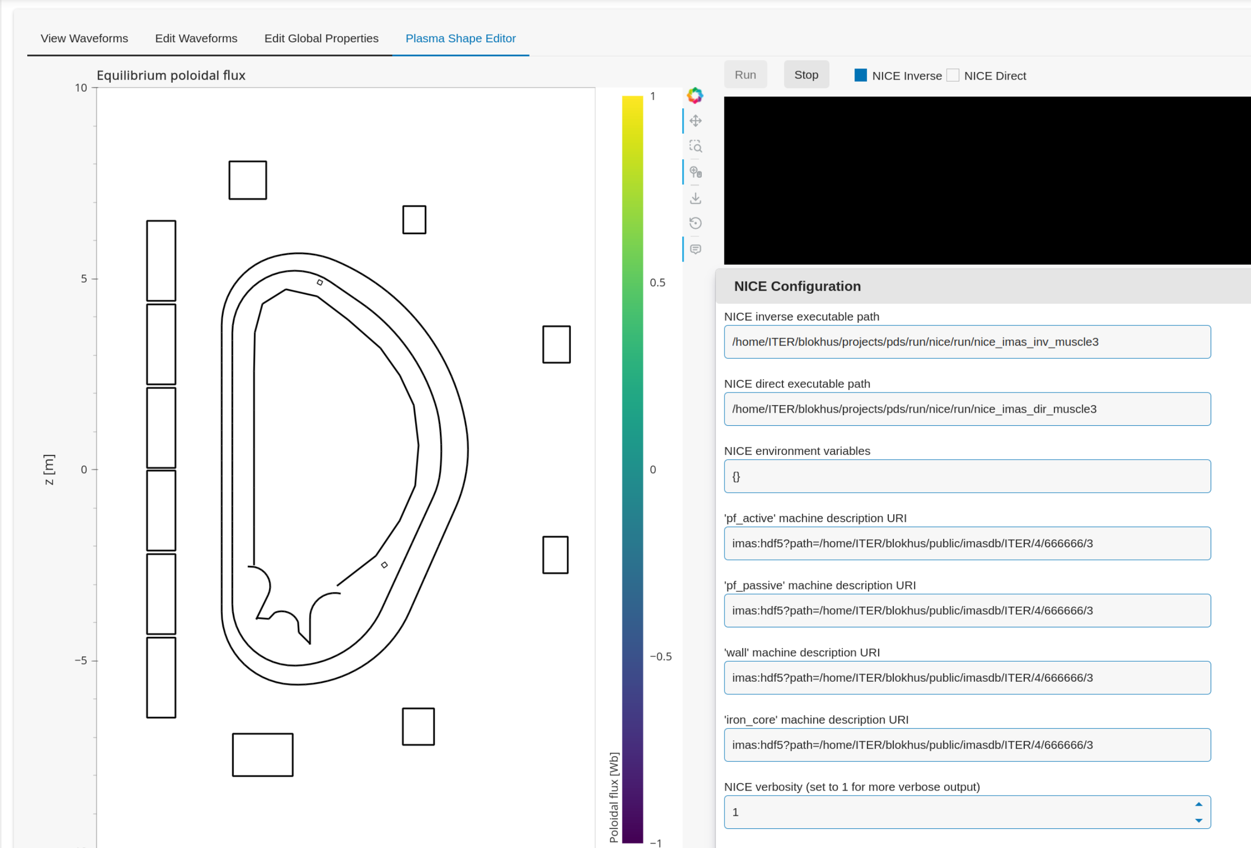
Open the tab Plasma Shape Editor in the Waveform Editor GUI. You should see an empty plotting window on your left, and an options panel on your right. NICE requires configuration to be set.

1. Set the executable paths for the NICE inverse and direct mode. If you are using the NICE module, you can leave these at their default values: nice_imas_inv_muscle3 and nice_imas_dir_muscle3 for the inverse and direct mode, respectively. If you manually compiled NICE, you must provide the paths to the executables you built in the installation instructions.

2. Set any NICE environment variables required to run NICE. This depends on your specific system. If you are on SDCC, you can leave this as is.

   If you are running waveform editor locally (not on SDCC), you may get errors stating that there were issues when loading shared libraries, you might need to set the LD_LIBRARY_PATH. You can set them using the following dictionary style format: {'LD_LIBRARY_PATH': '<paths>'}, replacing the <paths> (including angle brackets).

3. Provide the URIs for the different types of machine description IDS that NICE requires. You can provide your own, or if you are on SDCC you can try to use the following URI:

   imas:hdf5?path=/home/ITER/blokhus/public/imasdb/ITER/4/666666/3
   

What happens after you fill in the machine description URIs?

After you fill in the URIs of the machine description, you should see the outline of the coils, as well as the outlines of the first wall, divertor and vacuum vessel.

For example:

Besides the machine description URIs you provided in the previous exercise, NICE requires some extra input to run. We focus on the inverse mode of NICE for now. For this mode NICE requires the following:

• A desired plasma shape

• The plasma current

• Characteristics of the vacuum toroidal field; R0 and B0

• p' and ff' profiles

First, open the Plasma Shape options panel, set it to parameterized, and leave the shape settings on theirs defaults for now.

Secondly, open the Plasma Properties options panel, and set it to the Manual option. Leave the values at its default for now. This will set the plasma current, R0 and B0, and the ff' and p' profiles through a parameterisation using the alpha, beta, and gamma parameters. Leave the values at default for now.

You should now have set up enough to run NICE inverse mode, which you can verify by checking that there are no more ⚠️ icons besides the option panels, and that the Run button is enabled.

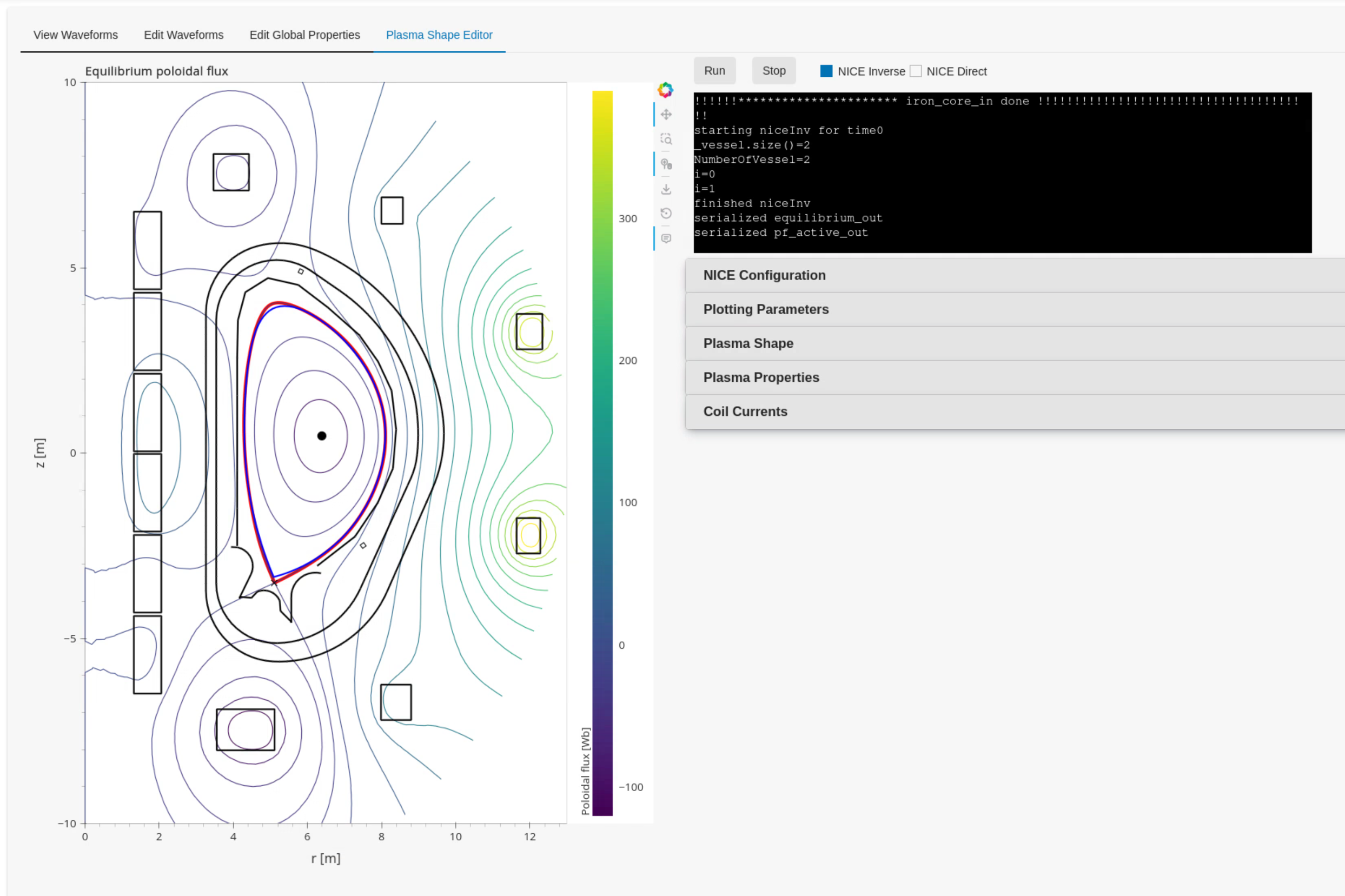
Run NICE by selecting the Run button.

What do you see in the plot on the left? What happens if you hover your mouse over the coil outlines? Change some of the parameters in the Plotting Parameters option panel. What do they do?

If NICE inverse converged with your desired plasma shape, you will see the resulting equilibrium contour lines appear on the plot on the left.

When you hover over the coil outlines, you will see the currents calculated by NICE.

Using the Plotting Parameters options, you can change how many contour lines are plotted, as well as change which plotting components are shown.

For example:

There are three ways to configure the desired plasma shape for NICE inverse in the Plasma Shape Editor.

1. By providing an equilibrium IDS containing a boundary outline.

2. By providing a geometric parameterization.

3. By providing gap distances for an equilibrium IDS containing boundary gaps.

We will cover the first two methods in this exercise.

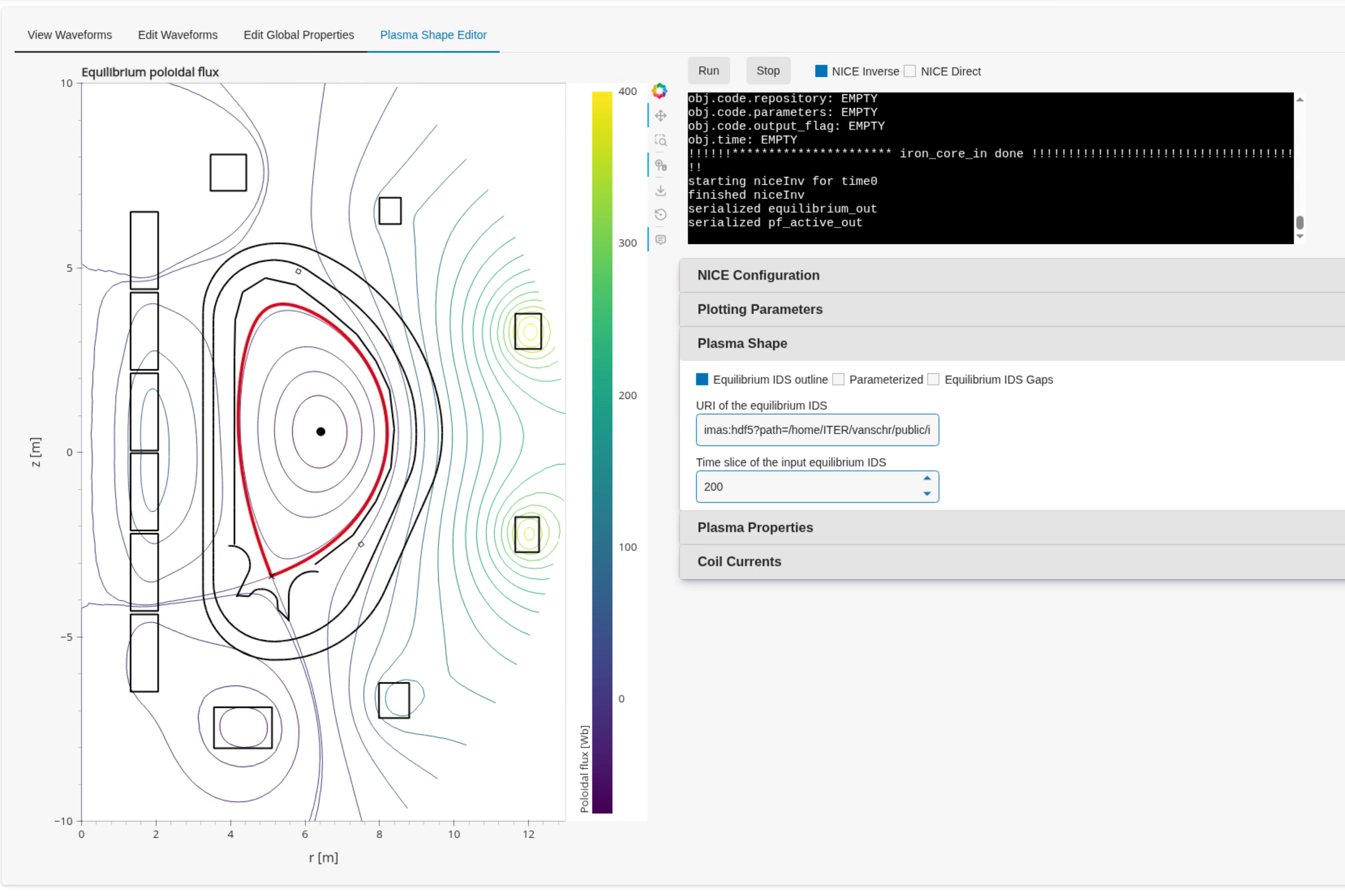
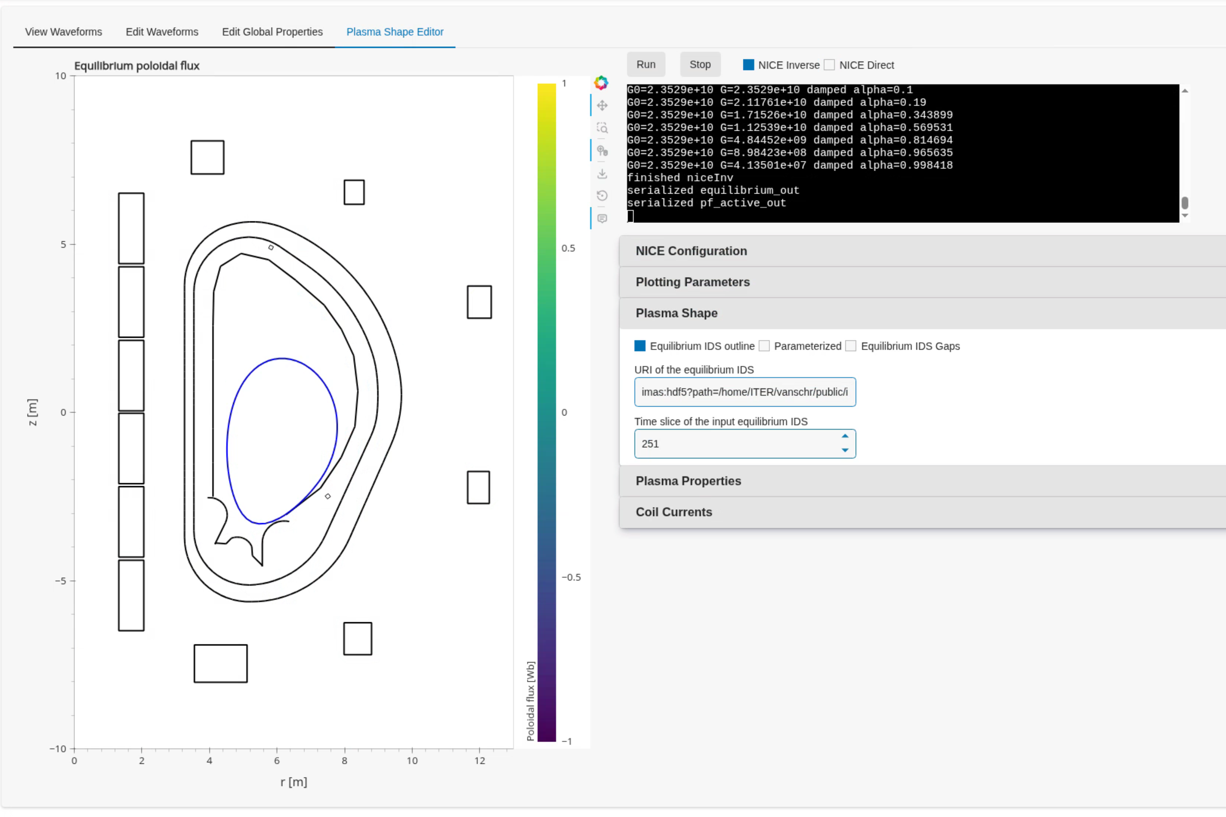
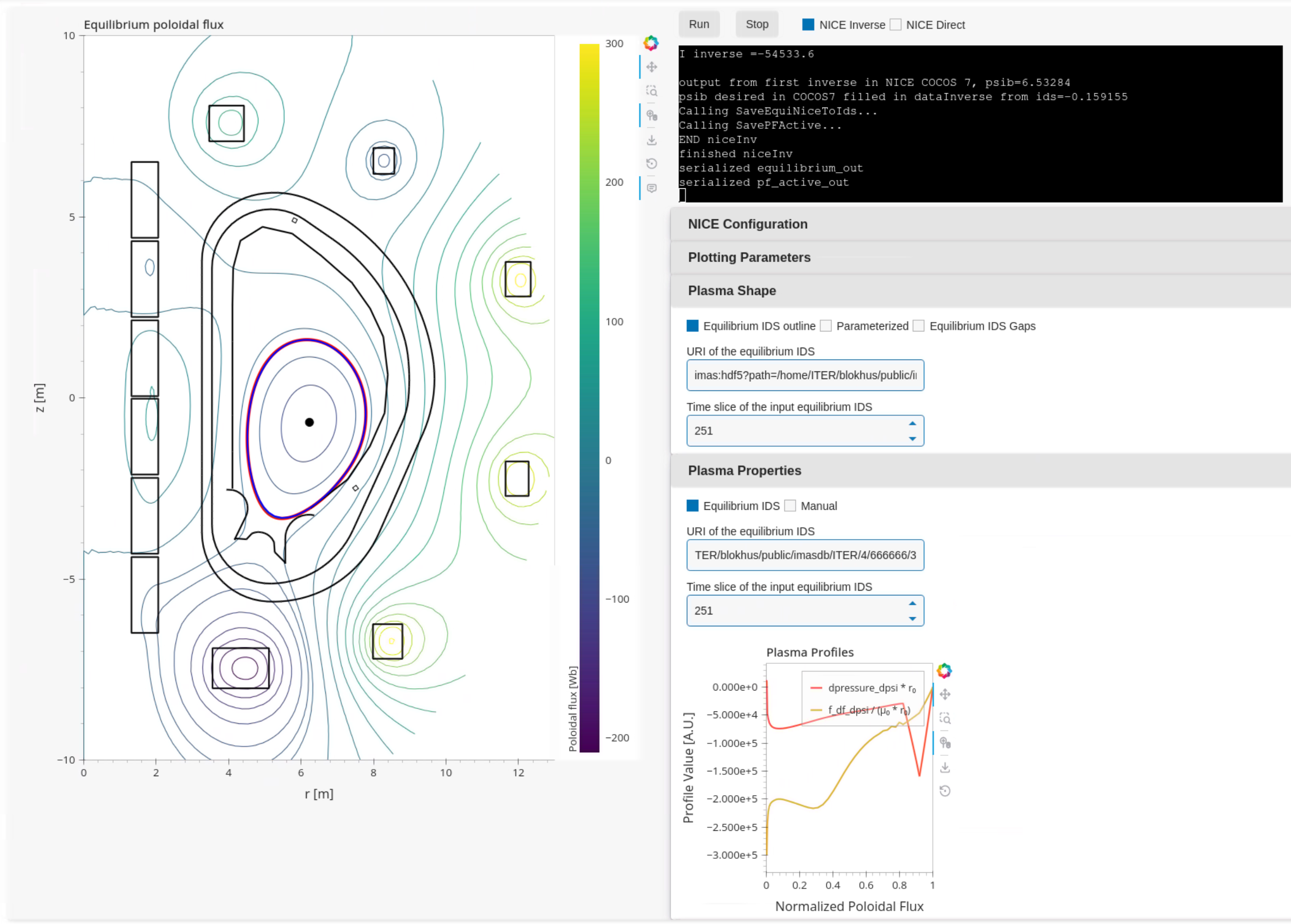
1. Select the Equilibrium IDS outline option. Provide an outline from an equilibrium IDS, for example by using the URI below if you are on SDCC. Visualize the boundary outline of the time steps at 200s and 251s, do you see a difference? Run NICE inverse for both time steps, what happens in each case? What happens if you change the P' and FF' profiles from the manual parameterisation to the profiles from the corresponding equilibrium IDS?

   imas:hdf5?path=/home/ITER/blokhus/public/imasdb/ITER/4/666666/3
   

2. Select the Parameterized option, and update some of the parameter sliders to change your desired shape. Run NICE in inverse mode, does it converge?

1. Running NICE inverse with time slice at 200s, converges and you should see the following equilibrium:

   

   Running it with the time slice at 251s with the default parameterised P' and FF' profiles, NICE doesn't converge and it will throw an error:

   

   However, if you use the P' and FF' profiles from the equilibrium IDS at 251s instead, NICE will converge:

   

2. If you provided a valid plasma shape NICE will converge and you will see the resulting equilibrium, otherwise you will receive an error. For example if the given shape cannot be achieved with the given input.

By default, NICE is able to freely change all coil currents to achieve the desired plasma shape. It is possible, however, you fix any of the coils to a specific value, and NICE will try to achieve your desired plasma shape by varying the unfixed coil currents. You can do this in the Coil Currents panel.

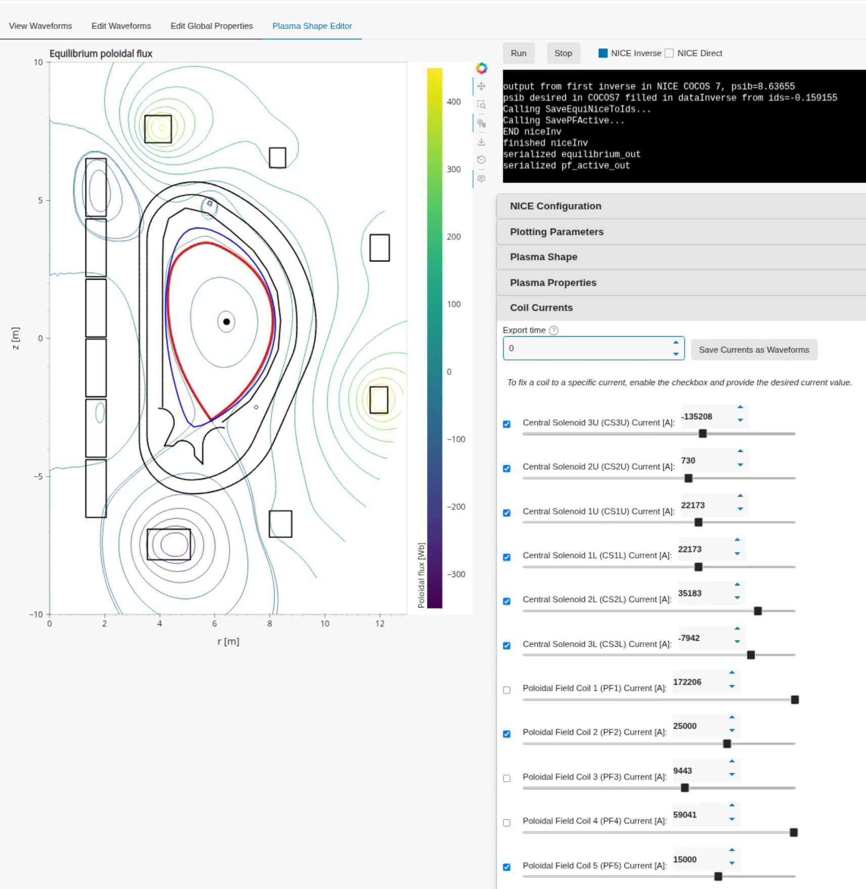
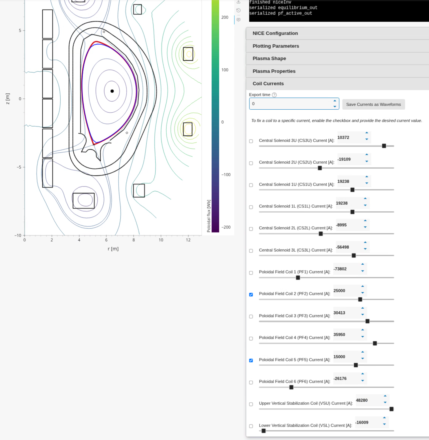
Load the plasma outline from previous exercise using the given IDS. Set the currents of PF2 and PF5 to 25000A and 15000A respectively, and enable the checkbox to fix the current. The sliders will update with the resulting coil currents after NICE inverse converges.

Did the currents of PF2 and PF5 stay fixed after running NICE?

Move some of the unfixed coil currents sliders randomly, and fix them. What happens?

After running NICE with PF2 and PF5 fixed, you will see that the unfixed coil currents change to get the desired plasma shape, for example:

If you fix too many coil currents, NICE is not able to represent the desired plasma shape anymore by changing the unfixed coil currents, and so NICE may not converge to the correct shape, for example: